Rethinking smoothness | Liuyuan Jiang

Summary

Penalty methods replace the lower-level optimality requirement with a penalty on its objective gap. Joint optimization then has a smoothness bound that grows with the penalty. This paper analyzes the objective obtained after lower-level minimization and proves that its smoothness bound stays of order $\mathcal O(1)$ , under the stated regularity conditions. The sharper bound gives $\mathcal O(\varepsilon^{-1})$ outer iterations for a squared projected-gradient tolerance $\varepsilon$ , with total work determined by the lower-level solver.

The reduced objective $F_\gamma$ has $\mathcal O(1)$ smoothness in $\gamma$ under the paper’s strong-convexity, Hessian, and constraint-regularity conditions. The proof compares directional curvatures of the original and perturbed value functions. Theorems 1 and 3
ALT-PBGD achieves $\mathcal O(\varepsilon^{-1})$ outer iterations for the squared projected-gradient tolerance $\varepsilon$ . Projected-gradient inner solves give $\widetilde{\mathcal O}(\varepsilon^{-1})$ total work under fixed lower constraints. Proposition 2
The coupled-constraint extension preserves the $\mathcal O(\varepsilon^{-1})$ outer rate. Total work is $\mathcal O(\varepsilon^{-2})$ with the specified general solver and $\widetilde{\mathcal O}(\varepsilon^{-1})$ in the affine-in-y, full-domain regime. Proposition 4 and Remark 1

A large joint penalty does not imply large reduced curvature

The smoothness bound that controls the step

The joint penalty objective $H_\gamma(x,y)$ measures changes in both variables. Its $\mathcal O(\gamma)$ smoothness bound leads to a penalty-dependent step size. ALT-PBGD and BLOCC instead update the upper variable using the reduced objective $F_\gamma(x)$ , after estimating the lower responses.

Cancellation between constrained value functions

The reduced objective is $\gamma$ times the difference between two related lower-level minimum values. Strong convexity controls the change in the lower response, and Hessian regularity controls the resulting change in directional curvature. Analyzing the difference preserves the cancellation of the penalty factor.

From smoothness to complexity

The $\mathcal O(1)$ reduced bound permits a step-size order independent of $\gamma$ . This gives $\mathcal O(\varepsilon^{-1})$ outer iterations for the squared projected-gradient criterion. The lower-level solver determines the additional cost within each iteration.

Alternating and primal-dual updates for the reduced objective

Solve two lower problems. ALT-PBGD estimates the minimizers of g and g + f/ $\gamma$ at the current upper variable. The first value anchors lower-level optimality. The second incorporates the upper objective.

Form the reduced gradient. The outer gradient combines the upper-objective gradient with the difference of the two lower-objective gradients. BLOCC adds the multiplier terms required by constraints that depend on x.

Take a projected upper step. The algorithms project the upper update onto X. The $\mathcal O(1)$ smoothness bound permits a penalty-independent step-size order, while the inner problems are solved to the accuracy required by the convergence analysis.

The penalty factor cancels after lower-level minimization

The lower problem defining $v_\gamma$ is a perturbation of the problem defining v by f/ $\gamma$ . Strong convexity keeps their responses close, and Lipschitz Hessians control the corresponding directional-curvature difference. The paper analyzes that difference as a single quantity. Multiplication by $\gamma$ then leaves an $\mathcal O(1)$ bound for the reduced objective.

Directional-curvature cancellation under constraints

Notation

$x,\;y$: Upper-level and lower-level variables.
$f(x,y),\;g(x,y)$: Upper-level and lower-level objectives, respectively.
$\gamma$: Penalty constant in the joint objective.
$\mathcal X,\;\mathcal Y,\;\mathcal Y(x)$: Upper domain, base lower domain, and lower feasible set depending on x.
$c(x,y)$: Vector of lower-level inequality constraints.
$v(x),\;v_\gamma(x)$: Original and perturbed lower-level minimum values. $y_g$ and $y_\gamma$ are the corresponding minimization variables.
$H_\gamma(x,y),\;F_\gamma(x)$: Joint penalty objective and its reduced objective after lower minimization.
$y_g^*(x),\;y_\gamma^*(x)$: Original and perturbed optimal lower responses.
$\lambda_g^*(x)$: Original lower-level constraint multiplier in Equation 7.
$d,\;D^2_{dd}$: Unit direction and second-order directional derivative along d.
$\eta,\;G_\eta(x)$: Outer step size and projected-gradient mapping, defined below.
$\varepsilon$: Tolerance for the squared generalized-gradient norm. Proj denotes Euclidean projection onto the indicated domain.

\mathcal Y(x)=\{y\in\mathcal Y:c(x,y)\leq0\}

v(x)=\min_{y_g\in\mathcal Y(x)}g(x,y_g)

H_\gamma(x,y)=f(x,y)+\gamma\bigl(g(x,y)-v(x)\bigr)

v_\gamma(x)=\min_{y_\gamma\in\mathcal Y(x)}\bigl[\gamma^{-1}f(x,y_\gamma)+g(x,y_\gamma)\bigr]

F_\gamma(x)=\gamma\bigl(v_\gamma(x)-v(x)\bigr)

The original value $v(x)$ minimizes g over $\mathcal Y(x)$ . The perturbed value $v_\gamma(x)$ minimizes g + f/ $\gamma$ over the same set. $H_\gamma(x,y)$ is the joint penalty objective, and $F_\gamma(x)$ is its minimum over the lower variable. The cancellation identity below compares directional derivatives along the unit direction d. The projected-gradient mapping $G_\eta(x)$ measures stationarity of $F_\gamma$ on the upper domain X.

\nabla v(x)=\nabla_xg(x,y_g^*(x))+\left\langle\lambda_g^*(x),\nabla_xc(x,y_g^*(x))\right\rangle

D^2_{dd}F_\gamma=\gamma\bigl[D^2_{dd}v_\gamma-D^2_{dd}v\bigr]

G_\eta(x)=\frac{x-\operatorname{Proj}_{\mathcal X}\!\left(x-\eta\nabla F_\gamma(x)\right)}{\eta}

Theorem 1 · Fixed feasible set

Cancellation in the reduced directional curvature

For sufficiently large $\gamma$ , the stated strong-convexity, gradient, Hessian, and constraint assumptions bound the second-order directional derivative of $F_\gamma$ by $\mathcal O(1)$ . Lemma 3 compares the curvatures of the two constrained value functions.

Theorem 1 · Fixed feasible set in the paper

Theorem 3 · Coupled feasible set

Regularity of the moving boundary

The coupled result adds a smooth boundary for Y and Lipschitz Hessians of the constraints. These conditions extend the directional-curvature comparison to a feasible set depending on x and yield $\mathcal O(1)$ smoothness for sufficiently large $\gamma$ .

Theorem 3 · Coupled feasible set in the paper

The constrained response supplies a replacement identity

At a constrained lower optimum, the lower-objective gradient need not vanish. For a fixed feasible set, Lemma 6 in the appendix shows that it is orthogonal to the directional change of the optimal response. This identity supports the directional-derivative comparison in Lemma 3.

Coupled constraints contribute a multiplier term

When $\mathcal Y(x)$ changes with x, Equation 7 expresses the value-function gradient through the lower response and its constraint multiplier. Theorem 3 extends the curvature comparison using regularity of the constraints and the domain boundary.

The convergence criterion belongs to the reduced objective

The mapping $G_\eta(x)$ is the projected gradient of $F_\gamma$ over X. Its squared norm is the criterion in Propositions 2 and 4. The lower-level approximation and the choice of $\gamma$ govern the penalty reformulation separately from this outer stationarity bound.

Assumptions behind the analysis

Assumptions 1–4 specify Lipschitz objective gradients, Lipschitz objective Hessians in the lower variable, strong convexity of g in that variable, closed convex domains, convex lower constraints, and linear independence of active constraint gradients. Theorems 1 and 3 establish $\mathcal O(1)$ reduced smoothness for sufficiently large $\gamma$ . The coupled-constraint result also uses Assumption 5: a smooth boundary for Y and twice-differentiable constraints with Lipschitz Hessians in the lower variable. Propositions 2 and 4 use the squared projected-gradient criterion ‖ $G_\eta(x)$ ‖² < $\varepsilon$ . Their $\mathcal O(\varepsilon^{-1})$ bound counts outer updates. The total bounds include approximate inner solves.

Theorems 1 and 3 · Reduced smoothness in the paper

Further details

How is the reduced gradient computed?

ALT-PBGD combines first-order gradients at the original and perturbed lower responses. BLOCC computes the corresponding primal-dual responses and includes constraint-gradient terms through their multipliers. Equations 14 and 17 give the updates.

What do the second-order derivatives do?

The Hessian and directional-derivative calculations establish the smoothness bound used in the convergence analysis. The analyzed algorithms compute the outer direction with first-order gradients and approximate lower-level solutions.

Related projects

This paper sharpens the smoothness analysis of BLOCC, the primal-dual penalty method for coupled constraints. Efficient Penalty-Based Bilevel Methods combines this analysis with updated algorithms and a flatness condition. PBGD-Free uses flatness to remove the original lower-response solve from the update.

BLOCC Efficient penalty methods PBGD-Free

Illustration

Joint curvature and reduced curvature

x is the upper variable, y is the lower variable, and $\gamma$ weights the lower-level penalty. Minimizing over y gives y = x. Move $\gamma$ to see the fixed slice steepen while the reduced curve stays in place.

\begin{aligned}H_\gamma(x,y)&=\frac{x^2}{2}+\gamma(y-x)^2\\F_\gamma(x)&=\min_y H_\gamma(x,y)=\frac{x^2}{2}\end{aligned}

Penalty

\gamma

Fixed slice

H_\gamma(x,0)

Reduced

F_\gamma(x)

Both axes stay fixed for every penalty setting. In this quadratic example, the fixed slice has curvature 1 + 2 $\gamma$ and the reduced objective has curvature 1.

The quadratic illustration

The plotted quadratic separates a fixed slice of the joint objective from the reduced curve after minimization over y. Increasing $\gamma$ steepens the fixed slice while leaving $F_\gamma$ unchanged. The paper’s Example 1 uses different, nonquadratic objectives to illustrate the same distinction.

Convergence and total solver complexity

Original EUSIPCO Table I comparing smoothness and total complexity across fixed, nonlinear coupled, and affine lower-level constraint regimes. — **Table I · The constraint regime changes the complexity**
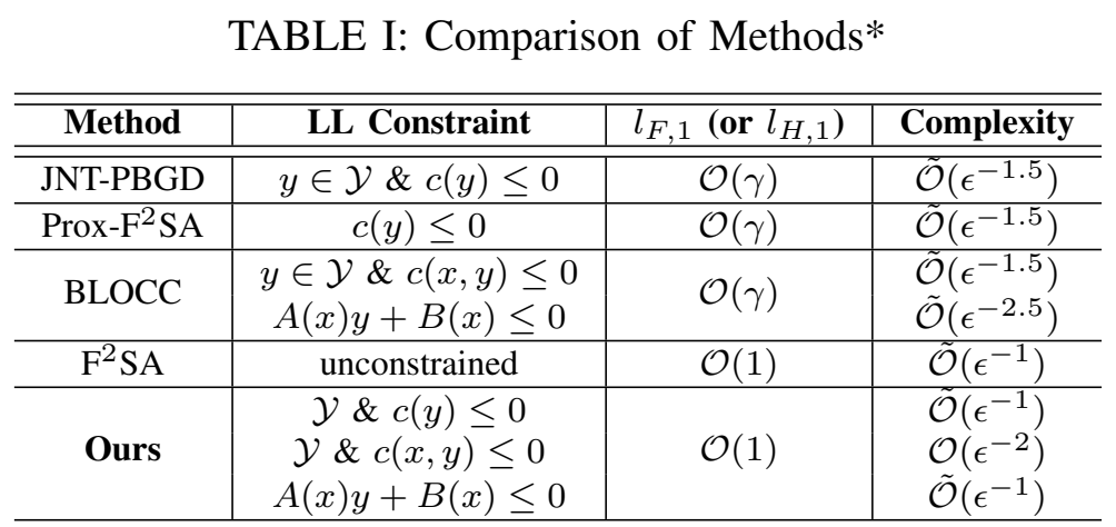
Table I separates fixed, general coupled, and affine-in-y constraints. The complexity column combines outer iterations with the work of the lower-level solver for each regime.
Original paper source

The objective being analyzed. Joint PBGD uses the $\mathcal O(\gamma)$ smoothness bound of H $\gamma$ . The reduced analysis of $F_\gamma$ gives $\mathcal O(1)$ smoothness under the paper’s assumptions.

The cost of the lower-level solver. Fixed, general coupled, and affine-in-y constraints lead to different total complexity bounds because the inner minimization or primal-dual solver has a different convergence rate.

The stationarity tolerance. Table I uses a squared generalized-gradient criterion. Õ suppresses logarithmic factors. The $\mathcal O(\varepsilon^{-1})$ outer count is separated from total work in Propositions 2 and 4.

ALT-PBGD under fixed lower constraints

Proposition 2 · squared projected-gradient tolerance $\varepsilon$
Update	Smoothness order	Outer iterations	Overall work
Joint PBGD	$\mathcal O(\gamma)$	$\mathcal O(\varepsilon^{-3/2})$	$\widetilde{\mathcal O}(\varepsilon^{-3/2})$
ALT-PBGD	$\mathcal O(1)$	$\mathcal O(\varepsilon^{-1})$	$\widetilde{\mathcal O}(\varepsilon^{-1})$

Result

The $\mathcal O(1)$ reduced smoothness bound allows a constant step-size order. Projected gradient descent solves each strongly convex inner problem with logarithmic work, giving $\widetilde{\mathcal O}(\varepsilon^{-1})$ total complexity for ALT-PBGD.

Experiment setup and comparison details

Assumptions 1–4 and a nonempty fixed closed convex lower feasible set. Theorem 1 applies for sufficiently large $\gamma$ . Proposition 2 measures ‖ $G_\eta(x)$ ‖² < $\varepsilon$ and counts $\mathcal O(\varepsilon^{-1})$ outer updates. The total bound uses projected gradient descent as the inner minimization solver. Õ suppresses logarithmic factors.

Read the original analysis

BLOCC under coupled lower constraints

Proposition 4 and Remark 1 · outer rate and total work
Lower-level constraints	Reduced smoothness	Outer iterations	Overall work
General nonlinear coupled	$\mathcal O(1)$	$\mathcal O(\varepsilon^{-1})$	$\mathcal O(\varepsilon^{-2})$
Affine in y; Y = ℝᵈ	$\mathcal O(1)$	$\mathcal O(\varepsilon^{-1})$	$\widetilde{\mathcal O}(\varepsilon^{-1})$

Result

The reduced smoothness bound gives $\mathcal O(\varepsilon^{-1})$ outer updates in both regimes. Remark 1 reports $\mathcal O(\varepsilon^{-2})$ total work with the accelerated MaxMin solver for general constraints and $\widetilde{\mathcal O}(\varepsilon^{-1})$ with the specified solver when the constraints are affine in y and the lower domain is the full space.

Experiment setup and comparison details

Assumptions 1–5, including strong convexity of the lower objective, constraint qualification, objective and constraint Hessian regularity, and a smooth domain boundary. The stationarity criterion is ‖ $G_\eta(x)$ ‖² < $\varepsilon$ . Proposition 4 gives the outer count; Remark 1 invokes the respective BLOCC inner solvers for the total bounds.

Read the original analysis

Work within each outer update

Each outer update computes the original and perturbed lower responses. Fixed constraints permit linearly convergent projected-gradient inner solves. Coupled constraints require primal-dual solves, whose cost depends on the constraint structure. These costs account for the different total complexity bounds below.

Cite this work

@inproceedings{jiang2025smoothness,
  title = {Improved Analysis of Penalty-Based Methods for Bilevel Optimization with Coupled Constraints},
  author = {Liuyuan Jiang and Quan Xiao and Tianyi Chen},
  booktitle = {2025 33rd European Signal Processing Conference (EUSIPCO)},
  year = {2025}
}

Summary

A large joint penalty does not imply large reduced curvature

The smoothness bound that controls the step

Cancellation between constrained value functions

From smoothness to complexity

Alternating and primal-dual updates for the reduced objective

The penalty factor cancels after lower-level minimization

Directional-curvature cancellation under constraints

Notation

Cancellation in the reduced directional curvature

Regularity of the moving boundary

The constrained response supplies a replacement identity

Coupled constraints contribute a multiplier term

The convergence criterion belongs to the reduced objective

Further details

Related projects

Joint curvature and reduced curvature

Joint curvature and reduced curvature

The quadratic illustration

Convergence and total solver complexity

ALT-PBGD under fixed lower constraints

BLOCC under coupled lower constraints

Work within each outer update

Cite this work

Research sources