BLOCC | Liuyuan Jiang

Summary

Coupled constraints make the lower-level feasible set depend on the outer variable. This changes the derivative of the lower-level value and can make joint feasibility projections expensive. BLOCC addresses both effects with a primal-dual penalty formulation: constraint multipliers enter the value gradient, and first-order updates use projections onto separate domains. The paper establishes finite-time convergence and evaluates the method on constrained SVM training and transportation network design.

In Figure 1, for a positive upper variable x, the multiplier-weighted constraint derivative changes the objective-only derivative −4x into the correct value gradient 2x. Lemma 2 · Figure 1
BLOCC uses first-order primal-dual subproblem solves and separate-domain projections. Including the inner solves, total iteration complexity is $\widetilde{\mathcal O}(\varepsilon^{-5/2})$ in the general regime and $\widetilde{\mathcal O}(\varepsilon^{-3/2})$ in the affine-in-y regime, where $\varepsilon$ is the target squared generalized-gradient tolerance. Theorems 2–4
On diabetes, Table 2 reports similar test accuracy for BLOCC and LV-HBA, with lower mean runtime for BLOCC under the reported stopping rule. Table 2
The Seville network experiment contains 49,216 variables and 13,336 constraints. BLOCC reaches convergence in the reported runs while LV-HBA exceeds the 24-hour limit. Table 3

Bilevel optimization on a moving feasible set

Coupled lower-level constraints

A transportation operator chooses link capacities, while passengers choose routes subject to those capacities. In the SVM application, hyperparameters bound the margin violations permitted during model fitting. Both problems have lower-level constraints that depend on the outer variable.

The boundary contributes to the derivative

The derivative of the minimum value $v(x)$ depends on how g changes and on how the feasible boundary moves. Omitting the second contribution can reverse the gradient, as Figure 1 demonstrates. The active constraints contribute through their optimal multipliers $\mu_g^*(x)$ .

A primal-dual penalty formulation

BLOCC penalizes the gap between g(x, y) and $v(x)$ and represents the coupled inequalities with a Lagrangian term. This gives two saddle-point problems whose primal-dual solutions determine the outer gradient. The resulting algorithm uses first-order derivatives and projections onto separate domains, avoiding a joint projection onto the coupled feasible set.

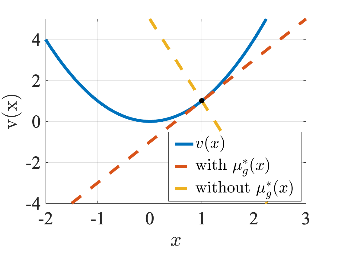
Original BLOCC Figure 1 comparing the value function with gradients computed with and without the constraint multiplier. — **Figure 1 · The missing constraint contribution**
In the paper’s example, the value-function gradient includes a Lagrange-multiplier term. Omitting that term can reverse the descent direction. This is why the coupled constraints enter BLOCC’s primal-dual formulation.
Original paper source

Constrained response. Figure 1 uses $g(x,y)=(y-2x)^2$ and $g^c(x,y)$ = 3x − y. For x > 0, the constraint $y\geq3x$ is active, giving $y_g^*(x)=3x$ and $v(x)=x^2$ .

Objective derivative. Evaluating the partial derivative $\nabla_x g$ at the constrained response gives −4x. The true derivative of $v(x)$ is 2x, so the objective term alone has the opposite sign.

Multiplier correction. The optimal multiplier is $\mu_g^*(x)=2x$ . Multiplying it by the constraint derivative contributes 6x, restoring the value gradient: −4x + 6x = 2x.

Two saddle-point solves per outer update

The original lower-level saddle problem. Approximate $y_g^*(x)$ and $\mu_g^*(x)$ to estimate the gradient of $v(x)$ , including the contribution from $g^c(x,y)$ .

The penalized saddle problem. Approximate $y_F^*(x)$ and $\mu_F^*(x)$ for the objective that combines f, the lower-level value-gap penalty, and the constraint Lagrangian.

The projected outer update. Combine the two primal-dual responses into the gradient estimate in Equation 13, then update x with a projection onto X. Inner updates project onto Y and the nonnegative multiplier domain.

Lower-level value gaps control response error

Lemma 1 bounds the squared distance to $y_g^*(x)$ by the gap g(x, y) − $v(x)$ for feasible y. The penalty therefore links the single-level formulation to lower-level optimality. Theorem 1 quantifies this approximation when $\gamma$ is chosen for the target response error.

Primal-dual reformulation and convergence

Notation

$x,\;y$: Upper-level and lower-level variables.
$f(x,y),\;g(x,y)$: Upper-level and lower-level objectives, respectively.
$\mathcal X,\;\mathcal Y,\;\mathcal Y(x)$: Upper domain, base lower domain, and coupled lower feasible set.
$g^c(x,y)$: Vector of coupled inequality constraints in Equation 1b.
$\mu$: Nonnegative multiplier vector for the coupled inequalities in Equation 2a.
$y_g^*(x),\;\mu_g^*(x)$: Original lower-level optimal response and its constraint multiplier.
$y_F^*(x),\;\mu_F^*(x)$: Primal-dual solution of the penalty subproblem in Equation 5.
$v(x)$: Original lower-level minimum value in Equation 2b.
$F_\gamma(x),\;\gamma$: Primal-dual penalty reformulation in Equation 2 and its penalty constant.
$\varepsilon$: Tolerance for the squared generalized-gradient stationarity criterion.

\mathcal Y(x):=\{y\in\mathcal Y:g^c(x,y)\leq0\}

y_g^*(x):=\operatorname*{arg\,min}_{y\in\mathcal Y(x)}g(x,y)

\min_{x\in\mathcal X}f\bigl(x,y_g^*(x)\bigr)

v(x)=\min_{y\in\mathcal Y(x)}g(x,y)

F_\gamma(x)=\max_{\mu\geq0}\min_{y\in\mathcal Y}\bigl[f(x,y)+\gamma(g(x,y)-v(x))+\langle\mu,g^c(x,y)\rangle\bigr]

The coupled constraint $g^c(x,y)$ defines the feasible set $\mathcal Y(x)$ . The lower-level response $y_g^*(x)$ minimizes g over that set, and $v(x)$ is the resulting minimum value. Equation 8 differentiates $v(x)$ using both the objective derivative and the multiplier-weighted constraint derivative.

\nabla v(x)=\nabla_x g(x,y_g^*(x))+\bigl\langle\mu_g^*(x),\nabla_x g^c(x,y_g^*(x))\bigr\rangle

Lemma 2

The lower-level value has a constraint-sensitive gradient

Under Assumptions 1–4 and bounded optimal multipliers, $v(x)$ is smooth. Its gradient includes both the partial derivative of g and the multiplier-weighted partial derivative of g^c. The boundary term is what restores the correct derivative in Figure 1.

Lemma 2 in the paper

Theorems 1–4

Approximation and finite-time convergence

Theorem 1 controls the squared distance from the penalized response to $y_g^*(x)$ . The outer criterion is an averaged squared generalized-gradient norm for $F_\gamma$ . Including the two inner saddle-point solves, the general analysis gives $\widetilde{\mathcal O}(\varepsilon^{-5/2})$ total iterations under Assumptions 1–5. For affine-in-y constraints, an unconstrained lower domain, and the singular-value conditions in Theorem 4, the inner solver converges linearly and total complexity is $\widetilde{\mathcal O}(\varepsilon^{-3/2})$ . The Õ notation suppresses logarithmic factors.

Theorems 1–4 in the paper

Quadratic growth survives the coupled constraints

Strong convexity of g and convexity of the lower constraints yield the value-gap bound in Lemma 1. This supplies the lower-level error measure for the penalty reformulation.

The gradient requires two primal-dual responses

The response of the original lower problem determines $\nabla v(x)$ . The response of the penalized problem determines the other terms in $\nabla F_\gamma(x)$ . Algorithm 1 approximates both before taking the outer step.

Inner accuracy enters the outer convergence bound

Theorem 2 separates outer progress from the error of the two saddle-point solves. Both inner error terms are multiplied by $\gamma$ ², so the subproblem tolerances must tighten as the penalty grows. Theorems 3–4 include these solves in the total complexity.

Assumptions behind the analysis

Assumptions 1–4 impose Lipschitz regularity, strong convexity of g in y, convexity of g^c in y, nonempty closed convex domains, lower-level feasibility, and linear independence of active constraint gradients in y (LICQ). Lemmas 2–3 also use bounded optimal multipliers. A sufficiently large $\gamma$ preserves strong convexity of the penalized inner objective. The general inner-solver analysis in Theorem 3 additionally uses Assumption 5 on dual curvature near the optimum. Theorem 4 treats constraints affine in y with Y equal to the full lower-variable Euclidean space and uniformly bounded, positive singular values of the constraint matrix. The outer objective can be nonconvex.

Section 3 · Value-function derivative and convergence in the paper

Further details

Why are two primal-dual problems solved?

The original lower-level problem provides $y_g^*(x)$ , $\mu_g^*(x)$ , and the value gradient. The penalized problem provides $y_F^*(x)$ and $\mu_F^*(x)$ . Their contributions appear together in Equation 9, which Algorithm 1 estimates before updating x.

Which projection does the formulation remove?

BLOCC avoids projecting the pair (x, y) onto the coupled feasible set. It retains projections onto the separate domains X and Y and onto the nonnegative multiplier domain.

What is the convergence target?

The analysis bounds the averaged squared generalized-gradient criterion of $F_\gamma$ . A separate approximation result controls the squared distance from the penalized lower response to $y_g^*(x)$ . The total complexity includes the inner work required to estimate both primal-dual responses.

Related projects

Smoothness of the Penalty Formulation for Bilevel Optimization later sharpens the curvature analysis of this framework. Efficient Penalty-Based Bilevel Methods extends that analysis and develops updates based on a flatness condition.

Rethinking smoothness Efficient penalty methods

Illustration

An active constraint can reverse the objective-only gradient

Figure 1 / exact lower-level example

Move the constraint, change the response

x is the upper variable and y is the lower response. The lower objective g is minimized subject to the inequality $g^c(x,y)\leq0$ .

\begin{aligned}g(x,y)&=(y-2x)^2\\g^c(x,y)&=3x-y\\y_g^*(x)&=\operatorname*{arg\,min}_{y\geq3x}(y-2x)^2=3x\end{aligned}

Upper-level variable x1.00

Unconstrained minimumConstrained response

The shaded region satisfies the paper’s constraint $g^c(x,y)\leq0$ . The optimum is $y_g^*(x)=3x$ , with $\mu_g^*(x)=2x$ . Moving the boundary adds a constraint contribution to the value gradient. This is an exact lower-level solve of the paper’s example.

Transportation network design at three scales

The network experiments choose link capacities while accounting for passenger responses. Table 3 compares 3- and 9-node synthetic networks with a 26-node Seville instance containing 49,216 variables and 13,336 constraints. With $\gamma$ = 4 and step size 1.6 × 10⁻⁴, BLOCC records runtime 6.70 × 10⁴ seconds and operator utility 138.78 on the Seville instance. LV-HBA does not reach convergence within the 24-hour limit on the 9-node or Seville instances. The transportation comparison uses LV-HBA as the baseline.

Constrained SVM training and transportation network design

SVM test accuracy on diabetes and fourclass

Table 2 · test accuracy · mean ± standard deviation
Method	Diabetes	Fourclass
BLOCC	0.767 ± 0.039	0.761 ± 0.014
LV-HBA	0.765 ± 0.039	0.748 ± 0.060
GAM	0.721 ± 0.047	0.715 ± 0.056

Result

On diabetes, BLOCC and LV-HBA have similar mean test accuracy, both with a reported standard deviation of 0.039. On fourclass, their means are 0.761 and 0.748. GAM has lower mean accuracy in both datasets.

Experiment setup and comparison details

Section 4.2 evaluates linear SVM hyperparameter optimization on diabetes and fourclass with $\gamma$ = 12. Figure 3 reports diabetes trajectories over 50 random train–validation–test splits. Appendix E.2 states that BLOCC and LV-HBA solve Equation 63, while GAM uses the formulation from its original paper because the matrix required by GAM can be singular. Table 2 reports means and standard deviations.

Read the original result

Runtime under the upper-objective stopping rule

Table 2 · runtime entries · mean ± standard deviation
Method	Diabetes	Fourclass
BLOCC	1.729 ± 0.529	1.922 ± 0.108
LV-HBA	2.899 ± 1.378	2.404 ± 0.795
GAM	8.752 ± 4.736	13.481 ± 0.970

Result

BLOCC has the lowest mean runtime in both reported datasets. The diabetes comparison with LV-HBA is about 40% lower, computed from 1.729 and 2.899. These values measure time until the upper-objective update is smaller than 10⁻⁵.

Experiment setup and comparison details

Table 2 uses the upper-objective update threshold of 10⁻⁵ and reports runtime means and standard deviations. Test accuracy is a separate reported metric. The SVM comparisons use the hyperparameters listed in Appendix E.2, including the different GAM formulation described there.

Read the original result

Outer progress and inner solution accuracy

The complexity bounds combine projected outer updates with the work needed to solve both primal-dual subproblems. The target is the averaged squared generalized-gradient criterion for $F_\gamma$ , together with the lower-level response approximation specified in Equation 4.

Cite this work

@inproceedings{jiang2024blocc,
  title = {A Primal-Dual-Assisted Penalty Approach to Bilevel Optimization with Coupled Constraints},
  author = {Liuyuan Jiang and Quan Xiao and Victor M. Tenorio and Fernando Real-Rojas and Antonio G. Marques and Tianyi Chen},
  booktitle = {Advances in Neural Information Processing Systems},
  volume = {37},
  year = {2024}
}

Summary

Bilevel optimization on a moving feasible set

Coupled lower-level constraints

The boundary contributes to the derivative

A primal-dual penalty formulation

Two saddle-point solves per outer update

Lower-level value gaps control response error

Primal-dual reformulation and convergence

Notation

The lower-level value has a constraint-sensitive gradient

Approximation and finite-time convergence

Quadratic growth survives the coupled constraints

The gradient requires two primal-dual responses

Inner accuracy enters the outer convergence bound

Further details

Related projects

An active constraint can reverse the objective-only gradient

Move the constraint, change the response

Transportation network design at three scales

Constrained SVM training and transportation network design

SVM test accuracy on diabetes and fourclass

Runtime under the upper-objective stopping rule

Outer progress and inner solution accuracy

Cite this work

Research sources