Efficient penalty methods

Summary

Penalty-based bilevel methods repeatedly solve a lower-level problem before updating the upper variable. This work identifies two ways to reduce that cost. An analysis of the objective after lower-level minimization permits outer step sizes that stay constant as the penalty increases. A flatness condition bounds the error from removing the original lower-level response computation. The resulting PBGD-Free method uses one tracking update with fixed constraints and retains a constrained inner solve when the feasible set depends on the upper variable.

After lower-level minimization, the penalty objective has a smoothness bound independent of the penalty under the fixed-set and coupled regularity conditions. This permits constant-order outer step sizes. Theorems 3.1 and 5.1
ALT-PBGD reaches the squared generalized-gradient target in $\mathcal O(\varepsilon^{-1})$ outer iterations, compared with $\mathcal O(\varepsilon^{-3/2})$ for the joint update. Each alternating step still computes two lower-level responses. Proposition 1
Flatness controls the bias from removing the original response. PBGD-Free uses one tracking update with fixed constraints and retains a constrained inner solve with coupled constraints. Its stationarity bounds include a flatness-dependent residual. Theorems 4.1 and 5.2
On the diabetes SVM benchmark, mean runtime is 0.17 seconds for PBGD-Free and 2.64 seconds for PBGD-BLOCC. Their mean test accuracies are 76.99% and 77.58%, respectively, across 20 random splits. Table 7

Which curvature governs an alternating penalty method?

A penalty changes the joint update

A bilevel problem selects an upper variable while the lower variable minimizes its own objective. A value-function penalty makes lower-level suboptimality costly. Its joint curvature grows with the penalty, so a joint gradient step requires a smaller step size as the penalty increases.

Lower-level minimization changes the outer geometry

An alternating method first computes a perturbed lower-level response. The objective followed by the outer update becomes a scaled difference of two nearby value functions. Their curvature terms cancel under the paper’s regularity conditions, giving a smoothness bound independent of the penalty. The analysis applies to a fixed lower feasible set and extends to a feasible set that depends on the upper variable.

One response can be removed under flatness

Forming the full reduced gradient still requires the original and perturbed responses. PBGD-Free keeps the perturbed response and replaces the full gradient by the upper partial gradient. The paper’s flatness condition controls the resulting omission bias. The fixed-set algorithm is fully single-loop. With coupled constraints, it retains a constrained inner solve and uses a multiplier-based surrogate for the convergence analysis.

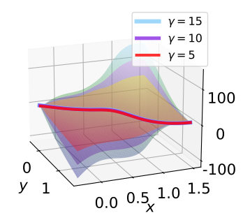
Original penalty-method Figure 3 comparing joint-gradient spheres and reduced-gradient lines for different penalty constants. — **Figure 3 · Joint gradients versus reduced gradients**
Example 3 compares the upper partial gradient of the joint penalty objective with the reduced-objective gradient at different penalty values. Evaluating along the optimized lower response reveals the cancellation analyzed by the reduced-smoothness theorems.
Original paper source

Joint upper partial gradients. The spheres show the upper partial gradient of the joint objective for different penalties. They depend on the current lower variable, which need not be an optimized response.

Reduced gradients. The lines show the gradient after lower-level minimization. Their dependence on the penalty is much smaller in Example 3.

The quantity analyzed. The reduced-smoothness theorems bound variation of the reduced gradient under their regularity assumptions. Figure 3 illustrates that geometry on one problem.

Alternating gradients and value-function-free updates

ALT-PBGD with a fixed feasible set. Compute the original and perturbed lower-level responses, then form the full reduced-penalty gradient. The penalty-independent smoothness bound permits an outer step size independent of the penalty.

PBGD-Free under flatness. Track only the perturbed response and update the upper variable with the upper partial gradient. Definition 11 controls upper-objective value variation relative to an original lower optimum and bounds the omitted correction.

Coupled-constraint updates. PBGD-BLOCC estimates two constrained primal-dual responses. The coupled PBGD-Free extension keeps the perturbed constrained solve and removes the original response computation. Its convergence analysis uses the multiplier-based surrogate in Equation 62.

Two improvements with different requirements

Reduced smoothness permits larger outer steps while retaining the full value-function correction. Removing that correction is a separate algorithmic change justified by flatness. The distinction determines both the stationarity quantity being controlled and the response work paid for at each iteration.

Reduced smoothness and generalized-gradient stationarity

Notation

$x,\;y$: Upper-level and lower-level variables, respectively.
$f(x,y),\;g(x,y)$: Upper-level and lower-level objectives.
$\gamma$: Positive penalty constant on the lower-level optimality gap.
$\mathcal X,\;\mathcal Y,\;\tilde{\mathcal Y},\;\mathcal Y(x)$: Upper domain, base lower domain, fixed feasible lower set, and lower feasible set depending on x.
$c(x,y)$: Vector of coupled lower-level inequality constraints.
$v(x),\;v_\gamma(x)$: Original and perturbed lower-level minimum values. The minimization variables are $y_g$ and $y_\gamma$ .
$y_g^*(x),\;y_\gamma^*(x)$: Minimizers of the original and perturbed lower-level objectives, respectively.
$\tilde F_\gamma(x,y),\;F_\gamma(x)$: Joint penalty objective and its reduction after lower-level minimization.
$\lambda_g^*(x)$: Optimal multiplier for the original coupled lower-level constraints.
$g^\lambda(x,y)$: Multiplier-based lower objective $g(x,y)+\langle\lambda_g^*(x),c(x,y)\rangle$ from Equation 52.
$F_\gamma^\lambda(x)$: Equation 62 surrogate formed from $g^\lambda(x,y)$ over the fixed base domain.
$c,\;\alpha,\;\delta(x),\;\delta$: Scalar flatness modulus, distance exponent, residual at x, and bound on the trajectory-average residual. The paper also uses c(x, y) for the separate vector constraint function.
$t,\;T$: Outer iteration index and number of outer iterations.
$\eta$: Outer step size in the projected update.
$G_{F_\gamma,\mathcal X}(x),\;G_{F_\gamma^\lambda,\mathcal X}(x)$: Generalized gradient mappings of the reduced objective and coupled surrogate on the upper domain. Their squared norms are the stationarity criteria in the convergence bounds.
$\epsilon$: Target accuracy for the squared generalized-gradient stationarity criterion.

\mathcal Y(x)=\{y\in\mathcal Y:c(x,y)\leq0\}

v(x)=\min_{y_g\in\mathcal Y(x)}g(x,y_g)

\tilde F_\gamma(x,y)=f(x,y)+\gamma\bigl(g(x,y)-v(x)\bigr)

v_\gamma(x)=\min_{y_\gamma\in\mathcal Y(x)}\bigl[\gamma^{-1}f(x,y_\gamma)+g(x,y_\gamma)\bigr]

F_\gamma(x)=\gamma\bigl(v_\gamma(x)-v(x)\bigr)

\bigl|f(x,y_g^*(x))-f(x,y)\bigr|\leq c\lVert y_g^*(x)-y\rVert^\alpha+\delta,\qquad\forall y\in\mathcal Y

g^\lambda(x,y)=g(x,y)+\langle\lambda_g^*(x),c(x,y)\rangle

F_\gamma^\lambda(x)=\min_{y\in\mathcal Y}\left[f(x,y)+\gamma\left(g^\lambda(x,y)-\min_{y\in\mathcal Y}g^\lambda(x,y)\right)\right]

The joint objective $\tilde F_\gamma(x,y)$ and the reduced objective $F_\gamma(x)$ describe different update geometries. ALT-PBGD differentiates the reduced objective using both lower-level responses. PBGD-Free retains the upper partial gradient and uses flatness to control the omitted correction. For coupled constraints, Theorem 5.2 analyzes the multiplier-based surrogate $F_\gamma^\lambda(x)$ defined in Equation 62.

Theorems 3.1 and 5.1

A penalty-independent smoothness bound

The joint penalty objective has smoothness order $\mathcal O(\gamma)$ , while the reduced objective $F_\gamma(x)$ has order $\mathcal O(1)$ . The fixed-set result uses lower-level strong convexity and objective regularity. The coupled result also uses bounded multipliers, strict complementarity, LICQ, and boundary regularity. Propositions 1 and 3 use this bound to obtain $\mathcal O(\varepsilon^{-1})$ outer iterations for squared generalized-gradient stationarity.

Theorems 3.1 and 5.1 in the paper

Theorems 4.1 and 5.2

Flatness determines the stationarity residual

The average squared generalized-gradient norm is bounded by $\mathcal O\!\left(T^{-1}+\delta^{\frac{2(\alpha-1)}{\alpha}}\right)$ under the theorem-specific step sizes and penalty choice. Theorem 4.1 measures this quantity for $F_\gamma(x)$ and analyzes a fully single-loop fixed-set update with 1 < $\alpha$ ≤ 1.5. Theorem 5.2 measures it for $F_\gamma^\lambda(x)$ , uses 1 < $\alpha$ < 1.5, and retains the constrained inner solve.

Theorems 4.1 and 5.2 in the paper

Cancellation between nearby value functions

The original and perturbed lower-level minimizers are separated by a distance of order $\mathcal O(\gamma^{-1})$ . Their second directional value derivatives differ by the same order under the regularity assumptions. Multiplying this difference by $\gamma$ therefore gives an $\mathcal O(1)$ curvature bound for $F_\gamma(x)$ . The directional derivatives handle constrained solution maps that need not admit an ordinary derivative. They are used in the analysis, while the algorithms use first-order information.

Why the penalty alone cannot justify dropping a response

The omitted term is a penalty-scaled difference of lower-objective upper gradients at the two responses. A response distance of order $\mathcal O(\gamma^{-1})$ can leave an order-one correction after multiplication by $\gamma$ . Example 1 gives opposite full and simplified gradient directions, and Proposition 2 bounds the resulting asymptotic error.

The role of Definition 11

Flatness bounds upper-objective value variation from $y_g^*(x)$ by a distance-power term plus a residual, for every lower variable in the base domain. Lemma 9 turns this value bound into a sharper response-distance bound. Lemma 10 controls the variation of the flatness residual along the outer trajectory. These bounds enter the PBGD-Free stationarity analysis.

A distinct surrogate for coupled constraints

The optimal lower multiplier defines $g^\lambda(x,y)$ by adding the coupled constraints to the lower objective. Equation 62 builds $F_\gamma^\lambda(x)$ from that objective over the fixed base domain. Lemma 16 compares its perturbed response with the constrained perturbed response used by the algorithm. Theorem 5.2 then bounds generalized-gradient stationarity for this surrogate, with the same flatness-residual order as the fixed-set result.

Assumptions behind the analysis

The fixed-set smoothness theorem uses a closed, convex, nonempty lower-level domain, lower-level strong convexity, jointly smooth objectives, upper-level Lipschitz continuity in the lower variable, and Hessians Lipschitz in the lower variable. The coupled extension adds Assumptions 3 and 5: constraints convex in the lower variable, LICQ near the lower optimum, bounded optimal multipliers, strict complementarity, a smooth boundary for the base domain, and constraint Hessian regularity. Theorem 4.1 assumes trajectory-wise flatness with 1 < $\alpha$ ≤ 1.5 and bounds the average squared generalized gradient of $F_\gamma(x)$ . Theorem 5.2 uses 1 < $\alpha$ < 1.5 and bounds the corresponding quantity for $F_\gamma^\lambda(x)$ . Both bounds contain a residual determined by average flatness along the trajectory.

Theorems 3.1, 4.1, 5.1, and 5.2 · HTML numbering in the paper

Further details

How do the preprint and conference papers differ?

The NeurIPS 2025 paper develops PBGD-Free under flatness. The EUSIPCO 2025 paper develops the reduced-smoothness analysis for constrained bilevel problems. This preprint brings those mechanisms together and analyzes the fixed-set single-loop algorithm and the coupled-constraint extension.

Why is a nearby perturbed response insufficient by itself?

The original and perturbed responses can be close while the penalty-scaled gradient difference stays of order one. Example 1 constructs opposing full and simplified directions. Flatness supplies the additional structure needed to bound the omission bias.

What does the stationarity residual measure?

The residual is part of an averaged squared generalized-gradient bound. It depends on the trajectory-average flatness residual and its exponent. The fixed-set and coupled theorems apply that criterion to different penalized objectives.

Related projects

The NeurIPS 2025 PBGD-Free paper develops value-function removal under flatness. The EUSIPCO 2025 smoothness paper studies the reduced-curvature mechanism. This preprint develops the fixed-set and coupled-constraint analysis together, including a fully single-loop fixed-set PBGD-Free method and the constrained extension.

PBGD-Free Rethinking smoothness BLOCC

Illustration

Fixed and coupled lower-level constraints

Method structure

Does the lower-level feasible set move?

Y is the base lower-level domain, $\tilde{\mathcal Y}$ is a fixed feasible set, and $\mathcal Y(x)$ is the feasible set at upper variable x. The inequalities $c(x,y)\leq0$ define coupled constraints. The update structure depends on whether these constraints move with x.

\mathcal Y(x)=\widetilde{\mathcal Y}

\mathcal Y(x)=\{y\in\mathcal Y:\ c(x,y)\leq0\}

Uncoupled constraints

Sections 4–5 analyze the update structure for fixed and coupled feasible sets.

Backbone adaptation and SVM hyperparameters

The LLM application assigns supervised fine-tuning to an output head and preference learning to LoRA backbone weights. After bilevel training, a new supervised head is fitted while the learned backbone stays fixed. The SVM application instead tunes per-example margin-violation bounds, which change the feasible set for the lower-level classifier. These tasks exercise the fixed-set and coupled-constraint update schedules.

Step sizes, response work, and constrained learning

Response computations in the analyzed methods

Algorithms 2–4 · fixed-set and coupled-constraint regimes
Method / regime	Inner work	Outer direction / condition
ALT-PBGD / fixed set	Original + perturbed response	Full reduced-penalty gradient
PBGD-Free / fixed set	One tracking update	Upper partial gradient; flatness
PBGD-BLOCC / coupled	Two primal-dual response solves	Multiplier-aware penalty gradient
PBGD-Free / coupled	Perturbed constrained inner solve	Flatness; surrogate analyzed in Theorem 5.2

Result

ALT-PBGD and PBGD-BLOCC form the full reduced-penalty gradient from two responses. PBGD-Free removes the original response computation. Its fixed-set theorem analyzes one perturbed-response tracking update per outer iteration. The coupled theorem keeps a constrained solve and measures stationarity for the multiplier-based surrogate.

Experiment setup and comparison details

Proposition 1 gives $\mathcal O(\varepsilon^{-1})$ outer iterations for ALT-PBGD versus $\mathcal O(\varepsilon^{-3/2})$ for JNT-PBGD under the fixed-set assumptions and the prescribed inner accuracy. Remark 6 includes the logarithmic cost of projected-gradient response solves. Proposition 3 gives $\mathcal O(\varepsilon^{-1})$ outer iterations for PBGD-BLOCC under Theorem 5.1. Remark 10 distinguishes general constrained inner-solver cost from the affine-in-the-lower-variable case. Theorems 4.1 and 5.2 add trajectory-wise flatness and bound averaged squared generalized-gradient stationarity with a residual.

Read the original analysis

Diabetes SVM: test accuracy and training time

Table 7 · diabetes · mean ± standard deviation
Method	Test accuracy ↑	Runtime (s) ↓
LV-HBA	0.7593 ± 0.0397	2.47 ± 0.23
GAM	0.7182 ± 0.0360	4.48 ± 0.22
BiC-GAFFA	0.7568 ± 0.0366	0.31 ± 0.01
PBGD-BLOCC	0.7758 ± 0.0292	2.64 ± 0.59
PBGD-Free	0.7699 ± 0.0313	0.17 ± 0.09

Result

PBGD-Free has the lowest reported mean runtime, 0.17 seconds, and PBGD-BLOCC has the highest reported mean test accuracy, 0.7758. PBGD-Free’s mean accuracy is 0.7699. The table reports standard deviations across the random splits.

Experiment setup and comparison details

The paper uses 20 random train–validation–test splits on the diabetes dataset. The upper variable sets margin-violation bounds and the lower problem trains a linear SVM. Runtime ends when the validation-loss change is below 10⁻⁵ or at 50 epochs. PBGD-Free uses penalty 20 and the coupled algorithm’s retained perturbed-response solve. Values are mean ± standard deviation.

Read the original result

Outer iterations and lower-level solver work

The complexity statements count outer iterations separately from the work inside a response solve. ALT-PBGD and PBGD-BLOCC estimate both the original and perturbed responses. PBGD-Free removes the original response computation. Its fixed-set version takes one tracking update per outer step, while its coupled version solves the remaining constrained subproblem to the prescribed accuracy.

Cite this work

@misc{jiang2025efficientpenalty,
  title = {Efficient Penalty-Based Bilevel Methods: Improved Analysis, Novel Updates, and Flatness Condition},
  author = {Liuyuan Jiang and Quan Xiao and Lisha Chen and Tianyi Chen},
  year = {2025},
  eprint = {2511.16796},
  archivePrefix = {arXiv}
}

Summary

Which curvature governs an alternating penalty method?

A penalty changes the joint update

Lower-level minimization changes the outer geometry

One response can be removed under flatness

Alternating gradients and value-function-free updates

Two improvements with different requirements

Reduced smoothness and generalized-gradient stationarity

Notation

A penalty-independent smoothness bound

Flatness determines the stationarity residual

Cancellation between nearby value functions

Why the penalty alone cannot justify dropping a response

The role of Definition 11

A distinct surrogate for coupled constraints

Further details

Related projects

Fixed and coupled lower-level constraints

Does the lower-level feasible set move?

Backbone adaptation and SVM hyperparameters

Step sizes, response work, and constrained learning

Response computations in the analyzed methods

Diabetes SVM: test accuracy and training time

Outer iterations and lower-level solver work

Cite this work

Research sources