PBGD-Free | Liuyuan Jiang

Summary

The gradient of a bilevel penalty objective depends on two lower-level responses: a minimizer of the original lower loss and a minimizer perturbed by the upper loss. PBGD-Free retains the perturbed response and removes the computation of the original response. A function-value flatness condition controls the omitted correction, giving a single-loop method with a quantified stationarity residual. The paper develops this analysis for nonconvex lower problems and evaluates the method in language-model fine-tuning.

PBGD-Free removes the original-response estimate from the penalty-gradient computation. With $K=1$ , one perturbed lower update and one upper update form each iteration. Equation 8 and Algorithm 1
The ( $\delta$ , $\alpha$ )-flatness condition bounds upper-loss variation from an original lower minimizer. Its residual $\delta$ and distance exponent $\alpha$ quantify the bias left by the omitted correction. Definition 1
Under the stated smoothness, PL, and flatness conditions, the average squared penalty-gradient norm decays as $\mathcal O(T^{-1})$ to a flatness-dependent residual. Theorem 3
Under a fixed training-time budget, PBGD-Free has the lowest reported DPO and SFT losses for Llama-3-3b, both at the trained outcome and after head adaptation with the backbone fixed. Table 2

Two lower-level responses in the penalty gradient

The original and perturbed lower problems

The paper studies an upper loss f evaluated at a minimizer of the lower loss g. Its penalty formulation adds the lower objective gap to f. The original response $y_g^*(x)$ minimizes g, while the perturbed response $y_\gamma^*(x)$ minimizes the joint penalty objective.

The cost of the value-function correction

Equation 5 differentiates the reduced penalty objective using both responses. Standard penalty updates therefore estimate two lower solutions before forming the outer direction. PBGD-Free removes the original-response estimate and retains the perturbed-response update.

Flatness controls the approximation error

The removed correction is multiplied by $\gamma$ , so its bias need not vanish as the penalty grows. The paper introduces a function-value flatness condition around an original lower minimizer, derives a sharper response-distance bound, and uses that bound to analyze the simplified updates.

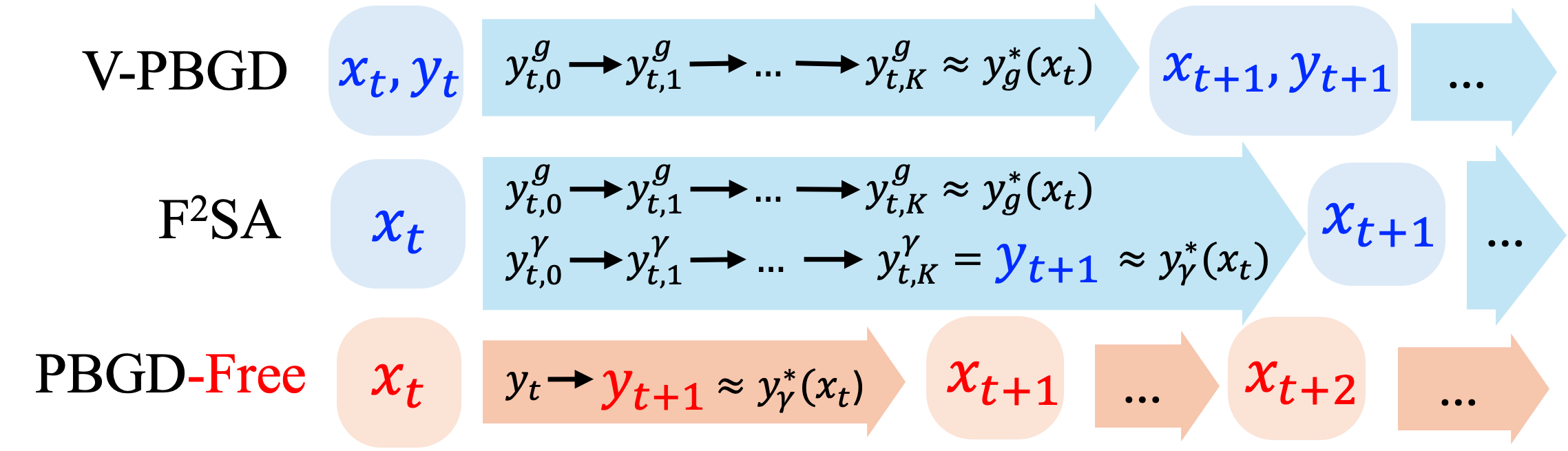
Original update comparison: V-PBGD and F2SA have inner refinements; PBGD-Free has one lower step followed by an upper step. — **Figure 1 · Single-loop update structure**
The diagram compares the original and perturbed response updates in V-PBGD and F2SA with PBGD-Free’s single-loop update. With $K=1$ , PBGD-Free takes one perturbed-response step followed by one upper-variable step. The flatness analysis bounds the omitted original-response correction.
Original paper source

Two response estimates. V-PBGD and F2SA use the original lower problem and the perturbed lower problem to assemble the penalty-gradient correction.

One retained response. PBGD-Free retains the perturbed lower iterate and updates the upper variable with $\nabla_x f$ . The fully single-loop version takes one tracking step per iteration.

Controlled omission bias. The update diagram identifies the computation removed by the method. Definition 1 and Theorem 3 supply the conditions and error bound for that omission.

A perturbed-response update without the value-function correction

Perturbed-response tracking. The lower iterate is warm-started from the preceding outer iteration and updated on $\gamma$ ⁻¹f + g.

Upper partial-gradient update. The upper variable is updated using $\nabla_x f$ evaluated at the tracked perturbed response. The original-response correction is omitted.

Single-loop specialization. Algorithm 1 permits K tracking steps. Theorem 3 analyzes $K=1$ , so each iteration uses one lower update and one upper update.

The removed response carries a gradient correction

Equation 5 expresses the reduced penalty gradient as the upper partial gradient plus a $\gamma$ -scaled difference of lower-loss gradients. Removing the original response saves its estimation cost. Flatness enters the analysis by controlling the distance between original and perturbed response sets, which bounds the omitted correction.

Flatness, penalty stationarity, and original-problem stationarity

Notation

$x,\;y$: Upper-level and lower-level variables.
$f(x,y),\;g(x,y)$: Upper-level and lower-level objectives, respectively.
$\gamma$: Penalty constant in Equation 2.
$\tilde F_\gamma(x,y),\;F_\gamma(x)$: Joint and reduced penalty objectives in Equation 2. z is the lower-variable dummy in the inner minimum.
$S_g^*(x),\;y_g^*(x)$: Set of lower-level minimizers of g and a solution in that set.
$S_\gamma^*(x),\;y_\gamma^*(x)$: Set of minimizers of the joint penalty objective and a solution in that set.
$c,\;\alpha,\;\delta$: Flatness modulus, distance exponent, and residual in Definition 1.
$t,\;T,\;k,\;K$: Outer-iteration index and budget, followed by lower-tracking-step index and budget.
$y_{t,k}^\gamma,\;y_t^\gamma$: Perturbed lower iterate during tracking and the iterate after K tracking steps.
$\eta,\;\eta^\gamma$: Outer and lower tracking step sizes in Algorithm 1.
$\delta(x_t),\;\delta$: Trajectory-dependent flatness residual and an upper bound on its average in Theorem 3.
$\varepsilon$: Target stationarity accuracy. Theorem 3 measures average squared penalty-gradient norm.
$d_x,\;d_y$: Dimensions of the upper and lower variables in the iterate-storage comparison in Table 1.

F_\gamma(x)=\min_y\tilde F_\gamma(x,y)=\min_y\left[f(x,y)+\gamma\left(g(x,y)-\min_z g(x,z)\right)\right]

\nabla F_\gamma(x)=\nabla_x f(x,y_\gamma^*(x))+\gamma\bigl[\nabla_x g(x,y_\gamma^*(x))-\nabla_x g(x,y_g^*(x))\bigr]

\delta

Definition 1 holds for all y: $y_g^*(x)$ is an original lower-level minimizer, $c\geq0$ is the modulus, $\alpha$ ≥ 1 is the distance exponent, and $\delta$ ≥ 0 is the permitted residual. The convergence theorem uses 1 < $\alpha$ ≤ 1.5 and a trajectory-dependent residual $\delta(x_t)$ . The perturbed minimizer $y_\gamma^*(x)$ minimizes the joint penalty objective, and $y_t^\gamma$ is its tracked iterate.

\frac1T\sum_{t=0}^{T-1}\lVert\nabla F_\gamma(x_t)\rVert^2\leq\mathcal O\!\left(T^{-1}+\delta^{\frac{2(\alpha-1)}{\alpha}}\right)

Proposition 2

A persistent bias under Lipschitz regularity

Proposition 2 constructs a bilevel problem satisfying Assumptions 1 and 2 where PBGD-Free retains a non-vanishing stationarity residual. The correction contains information about the dependence of the lower solution on x.

Proposition 2 in the paper

Theorem 3

Single-loop convergence under flatness

Under Assumption 2, a common exponent 1 < $\alpha$ ≤ 1.5, bounded modulus, the trajectory-average flatness bound, and the stated penalty and step sizes, $K=1$ gives the displayed bound on average squared penalty-gradient norm. Each iteration has constant first-order work. When the residual meets the target tolerance, the decaying term reaches that tolerance in $\mathcal O(\varepsilon^{-1})$ iterations.

Theorem 3 in the paper

Bias can persist as the penalty grows

The original and perturbed responses become close as $\gamma$ increases, but their lower-loss gradient difference is multiplied by $\gamma$ . Proposition 2 constructs a problem where the resulting stationarity residual remains nonzero. In Example 1, the full direction converges to x = −5, while the simplified upper partial-gradient direction converges to x = 0.

Flatness strengthens the response bound

Definition 1 measures upper-loss variation relative to an original lower minimizer for all y. The residual $\delta$ allows variation near that reference, and the exponent $\alpha$ controls the distance contribution. For 1 < $\alpha$ ≤ 1.5, Lemma 1 improves the bounds on the response-set distance and on the gap between the original hyper-objective and $F_\gamma$ .

Penalty stationarity and original-problem stationarity

Theorem 3 bounds the average squared gradient norm of $F_\gamma$ by a decaying iteration term and a flatness-dependent residual. Lemma 3 then relates a stationary point of $F_\gamma$ to an approximate KKT point of the original bilevel problem, with the penalty and flatness residual chosen for the target accuracy.

Single-loop update

y_{t,k+1}^{\gamma}=y_{t,k}^{\gamma}-\eta^{\gamma}\bigl[\gamma^{-1}\nabla_y f(x_t,y_{t,k}^{\gamma})+\nabla_y g(x_t,y_{t,k}^{\gamma})\bigr]

x_{t+1}=x_t-\eta\nabla_x f(x_t,y_t^{\gamma})

Equation 8 updates the perturbed lower iterate $y_{t,k}^\gamma$ and then x_t. Algorithm 1 uses K tracking steps and denotes the resulting lower iterate by $y_t^\gamma$ . Theorem 3 sets $K=1$ . The upper direction is $\nabla_x f$ , with no original-response estimate.

Assumptions behind the analysis

Assumption 2 requires smooth f and g, Lipschitz Hessians, and a uniform Polyak–Łojasiewicz inequality in y for the scaled upper/lower combinations specified there. Theorem 3 uses $K=1$ , a common flatness exponent 1 < $\alpha$ ≤ 1.5 and bounded modulus along the trajectory, the stated penalty choice, and the step-size conditions. Its criterion is the average squared gradient norm of $F_\gamma(x)$ , with a residual determined by the average flatness parameter. The proof gives the compatible outer and lower step sizes in Equation 63. Lemma 3 separately relates penalty stationarity to approximate KKT stationarity of the original bilevel problem under its accuracy conditions.

Assumption 2 · Definition 1 · Theorem 3 in the paper

Further details

What does the flatness condition measure?

Definition 1 bounds upper-loss variation relative to an original lower minimizer for all y. The modulus c and exponent $\alpha$ control its distance dependence, while $\delta$ permits a residual variation. This is a condition on function values, and its parameters enter the stationarity bound.

Which stationary objective does the theorem use?

Theorem 3 uses the average squared gradient norm of the reduced penalty objective $F_\gamma$ . Lemma 3 separately transfers a sufficiently accurate penalty stationary point to approximate KKT stationarity of the original bilevel problem under its penalty and flatness-accuracy conditions.

How are constrained lower problems handled?

The PBGD-Free paper analyzes the unconstrained lower problem. The efficient-penalty preprint develops fixed-set and coupled-constraint extensions. Its coupled-constraint method retains an inner solve for the constrained response.

Related projects

The efficient-penalty preprint extends the curvature analysis and flatness-based updates to fixed-set and coupled-constraint bilevel problems.

Efficient penalty methods Rethinking smoothness BLOCC

Illustration

Upper-loss variation relative to a lower minimizer

Definition 1 / illustrative envelope

How does the flatness bound shrink?

In Definition 1, $y_g^*(x)$ is a lower-level optimum for the fixed upper variable x. The modulus c, exponent $\alpha$ , and residual $\delta$ define the bound. Use the distance $\lVert y_g^*(x)-y\rVert$ directly. The green curve evaluates its right-hand side with the constants below; the blue curve shows the distance itself for comparison.

c=1,\qquad\alpha=1.5,\qquad\delta=0.003

Distance to the lower-level optimum0.10

Distance to optimumFlatness upper bound

The residual sets the envelope’s floor as the distance approaches zero.

Preference learning and head adaptation

In the application, x contains LoRA weights in the attention backbone and y is the output head. The upper loss is direct preference optimization (DPO), and the lower loss is supervised fine-tuning (SFT). A second evaluation phase freezes the learned backbone and adapts the head on another SFT dataset, measuring supervised adaptation together with the retained preference loss.

Preference learning with a reusable backbone

Preference and supervised losses at the trained outcome

Table 2 · outcome (xT, yT) · losses ↓
Method	Evaluated DPO	Evaluated SFT
V-PBGD	0.8180	1.0309
BOME	0.8332	1.1552
ALRIGHT	0.8055	0.8656
PBGD-Free	0.7837	0.8516

Result

PBGD-Free gives evaluated DPO loss 0.7837 and evaluated SFT loss 0.8516, the lowest values in these columns. ALRIGHT gives 0.8055 and 0.8656. The comparison evaluates the two losses under the same training-time budget, with ALRIGHT using a bi-objective formulation.

Experiment setup and comparison details

LoRA adaptation of the model labeled Llama-3-3b in the paper. DPO uses Dahoas/rm-hh-rlhf and SFT uses OpenOrca, with 4,800 samples per dataset and batch size 32. Appendix C.3 specifies LoRA rank 16 and alpha 16, Adam with learning rate 10⁻⁵, and NVIDIA A100 GPUs with 40 GB memory. Methods share a fixed training-time budget and complete different numbers of updates. Table 2 reports point estimates.

Read the original result

Head adaptation with the learned backbone fixed

Table 2 · post-SFT outcome (xT, ỹ) · losses ↓
Method	Evaluated DPO	Training SFT
V-PBGD	0.8423	0.9533
BOME	0.8402	0.9842
ALRIGHT	0.8201	0.7855
PBGD-Free	0.8088	0.6688

Result

After head adaptation, PBGD-Free gives evaluated DPO loss 0.8088 and training SFT loss 0.6688, compared with 0.8201 and 0.7855 for ALRIGHT. The SFT measure in this phase is a training loss. Its DPO measure evaluates preference loss with the adapted head.

Experiment setup and comparison details

Phase S2 freezes the learned backbone and adapts the head on another SFT dataset under a fixed-time budget. Table 2 reports the resulting evaluated DPO and training SFT losses as point estimates. The paper separately assesses generated output with BLEU and preference alignment with reward-gap and win-rate measurements.

Read the original result

Stationarity and first-order cost

Theorem 3 bounds the average squared gradient norm of the reduced penalty objective by an $\mathcal O(T^{-1})$ term plus a flatness-dependent residual. With that residual at the target tolerance, the deterministic method needs $\mathcal O(\varepsilon^{-1})$ iterations, each with constant first-order work. Lemma 3 gives the separate accuracy conditions for transferring penalty stationarity to the original bilevel problem.

Cite this work

@inproceedings{jiang2025pbgdfree,
  title = {Beyond Value Functions: Single-Loop Bilevel Optimization under Flatness Conditions},
  author = {Liuyuan Jiang and Quan Xiao and Lisha Chen and Tianyi Chen},
  booktitle = {Advances in Neural Information Processing Systems},
  volume = {38},
  year = {2025}
}

Summary

Two lower-level responses in the penalty gradient

The original and perturbed lower problems

The cost of the value-function correction

Flatness controls the approximation error

A perturbed-response update without the value-function correction

The removed response carries a gradient correction

Flatness, penalty stationarity, and original-problem stationarity

Notation

A persistent bias under Lipschitz regularity

Single-loop convergence under flatness

Bias can persist as the penalty grows

Flatness strengthens the response bound

Penalty stationarity and original-problem stationarity

Further details

Related projects

Upper-loss variation relative to a lower minimizer

How does the flatness bound shrink?

Preference learning and head adaptation

Preference learning with a reusable backbone

Preference and supervised losses at the trained outcome

Head adaptation with the learned backbone fixed

Stationarity and first-order cost

Cite this work

Research sources