SURF | Liuyuan Jiang

Summary

Linear scalarization converts competing objectives into a weighted optimization problem, but equal increments in the weight generally produce unequal distances along the Pareto front. SURF corrects this mismatch by estimating cumulative arc length and selecting weights at equal distance quantiles. The scalarized inner solver remains unchanged.

Nonuniform traversal speed explains why uniform scalarization weights generally produce uneven Pareto-front coverage. Integrating that speed gives an arc-length CDF whose inverse specifies the sampling weights. Geometry
SURF alternates warm-started scalarized optimization with monotone CDF reconstruction. It changes weight allocation while retaining the chosen inner solver. Algorithm 1
For N front segments, Assumptions 1–3 and the stated parameter and inner-solver conditions give linear convergence of CDF and optimization error to an $\mathcal O(N^{-2})$ discretization floor. The resulting coefficient of variation (CV) of neighboring gaps is $\mathcal O(N^{-1})$ . Theorem 1
For six Qwen2.5-0.5B summarization adapters with the same 12-epoch per-slot PPO budget, spacing CV falls from 0.65 ± 0.12 to 0.30 ± 0.17, while hypervolume rises from 3.76 ± 0.31 to 4.03 ± 0.35. Table 2

Why uniform weights produce uneven coverage

The coverage problem

Linear scalarization solves a weighted sum of competing objectives. Sweeping the weight produces a set of trade-offs, but evenly spaced weights need not produce evenly spaced objective vectors. A fixed computational budget can therefore yield dense clusters of similar solutions and leave other regions of the Pareto front sparsely represented.

The geometric cause

The scalarization optimum moves along the front at a speed that depends on the weight. Equal weight intervals represent unequal objective-space distances whenever that speed varies. The central question is how to allocate a finite set of scalarized solves so that their solutions cover the front uniformly.

Geometry-aware weight allocation

SURF measures coverage by arc length. Its normalized arc-length CDF maps a weight to the fraction of the front traversed. Equal quantiles of the inverse map give equally spaced solutions when the map is known. For general problems, SURF alternates finite, warm-started scalarized solves with monotone reconstruction of the map.

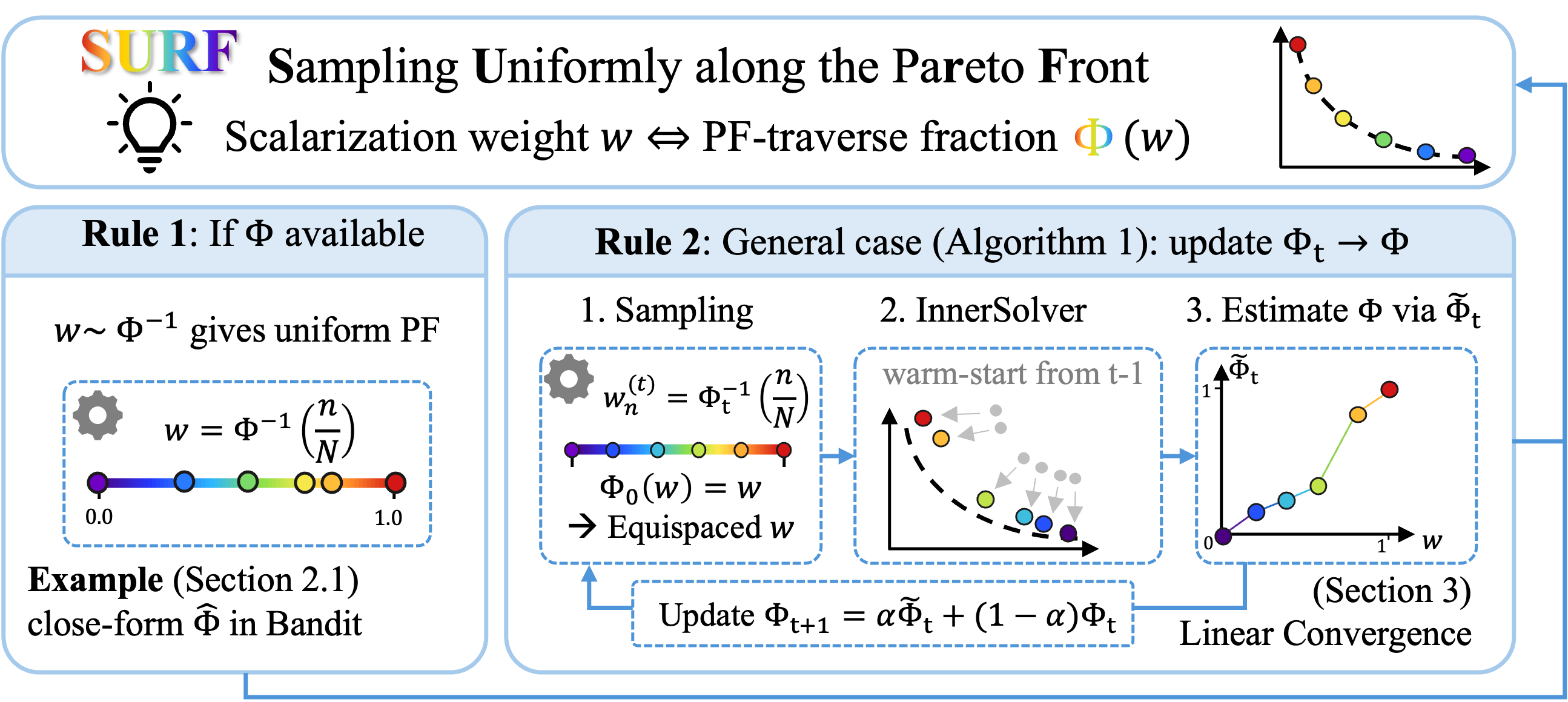
Original SURF overview showing the known-CDF rule and the iterative sampling, inner-solver, and CDF-estimation rule. — **Figure 2 · The SURF procedure**
SURF connects weights to arc length through a CDF. When the map is known, it is inverted directly; otherwise the method alternates between scalarized solves and CDF reconstruction.
Original paper source

Weight-to-front map. Each scalarization weight identifies an optimum and its objective vector. The CDF records the fraction of front arc length reached by that weight.

Analytical and estimated CDFs. Rule 1 uses a known CDF directly. Algorithm 1 implements Rule 2 by reconstructing the CDF from a finite set of solved points.

Refinement with finite inner solves. After the CDF update, each slot receives a revised weight and continues training from its preceding iterate. The inner solver and its optimization objective retain their scalarized form.

Arc-length reconstruction and weight refinement

Weight allocation. The current CDF estimate assigns each solution slot a weight at an equal quantile.

Warm-started optimization. Each slot continues its scalarized optimization from the previous iterate for a finite inner-solver budget.

Arc-length reconstruction. Distances between neighboring objective vectors define cumulative chord lengths. Monotone interpolation and a damped update refine the CDF estimate.

Scalarization geometry and convergence of SURF

Notation

$w$: Scalarization weight in [0, 1]; the two objective weights are w and 1 − w.
$\mathbf f_{\mathrm{PF}}(w)$: Objective vector at a scalarized optimum, defining the front path in Equation 4.
$v(w)$: Speed of that path in objective space.
$s(w)$: Cumulative arc length from weight 0 to w. In the integral, p is a dummy weight variable.
$\Phi(w)$: Normalized arc length $s(w)$ /s(1), the CDF in Equation 5.
$N,\;n$: N front segments give $N+1$ solution slots indexed by n = 0, …, N.
$\Phi_t,\;\tilde\Phi_t$: Current CDF estimate and the reconstructed CDF at outer iteration t.
$\alpha$: Damping parameter for the CDF update in Algorithm 1.

\begin{aligned}v(w)&=\left\lVert\frac{\partial\mathbf f_{\mathrm{PF}}(w)}{\partial w}\right\rVert\\s(w)&=\int_0^w v(p)\,dp\end{aligned}

\Phi(w)=\frac{s(w)}{s(1)}

w_n=\Phi^{-1}\!\left(\frac nN\right),\qquad n=0,\ldots,N

The path $\mathbf f_{\mathrm{PF}}(w)$ in Equation 4 records the objective vector at a scalarized optimum. Equation 5 defines its speed $v(w)$ , cumulative arc length $s(w)$ , and normalized map $\Phi(w)$ . Rule 1 inverts Φ at $n/N$ to obtain $N+1$ solutions separated by equal arc length.

\Phi_{t+1}=(1-\alpha)\Phi_t+\alpha\,\widetilde\Phi_t

Lemma 1

An invertible arc-length map

Under Assumptions 1–3, the Pareto-front traversal speed has finite positive lower and upper bounds. Consequently, s and Φ are strictly increasing, and Rule 1 can invert Φ to assign equal arc-length gaps.

Lemma 1 in the paper

Theorem 1

Linear convergence to the discretization floor

Under Assumptions 1–3, with sufficiently many segments, $\alpha\leq0.5$ , and the inner-solver budget of Remark 1, the combined CDF and hidden-space optimization error contracts by $1-\alpha/4$ per outer iteration toward $\mathcal O(N^{-2})$ . Equation 16 connects this estimate to spacing CV = $\mathcal O(N^{-1})$ .

Theorem 1 in the paper

Regularity of the scalarization path

Hidden strong convexity gives a unique optimum for each weight. Constraint regularity makes the optimum vary smoothly, and the nonzero-trade-off condition prevents the objective-space path from stopping. Lemma 1 consequently bounds $v(w)$ above and away from zero, making Φ strictly increasing and invertible.

From traversal speed to equal arc length

Equation 5 integrates the speed $v(w)$ into $s(w)$ and normalizes it into $\Phi(w)$ . The inverse rule $w_n=\Phi^{-1}(n/N)$ makes every neighboring pair span the same arc length s(1)/N. When Φ is unknown, Algorithm 1 estimates it from neighboring solved objective vectors and updates $\Phi_t$ using damping $\alpha$ .

CDF convergence and spacing uniformity

Theorem 1 controls both CDF reconstruction error and inexact inner optimization. Under its conditions, their combined measure contracts geometrically to an $\mathcal O(N^{-2})$ discretization floor. Equation 16 and Appendix E.3 then give CV = $\mathcal O(N^{-1})$ , connecting estimation accuracy to the variation in neighboring gaps.

Assumptions behind the analysis

Theorem 1 assumes a strongly convex hidden-space representation, fixed active constraints satisfying LICQ, a Lipschitz-continuous Lagrangian Hessian, and a nonzero projected trade-off throughout the scalarization path. These are Assumptions 1–3. With sufficiently many segments, $\alpha\leq0.5$ , and the inner-solver budget in Remark 1, the combined CDF sup-norm error and $C(N)$ -weighted maximum hidden-space solution error contracts by a factor $1-\alpha/4$ per outer iteration toward $\mathcal O(N^{-2})$ , with $C(N)=\Theta(N)$ . Equation 16 and Appendix E.3 relate this bound to spacing CV = $\mathcal O(N^{-1})$ after sufficiently many outer iterations.

Section 3 · Algorithm 1 and Theorem 1 in the paper

Further details

Which geometry defines uniform coverage?

Coverage is uniform in arc length under the chosen objective-space metric. Changing objective units or normalization changes the metric and the weights selected by the inverse CDF.

What is controlled in the quadratic example?

Appendix F.1 fixes the evaluation front while a gear parameter changes the scalarization-induced traversal speed. The interactive example uses the exact scalarized optimum and numerical integration of the arc-length map, so the curve stays fixed while the sampled weights change.

Related projects

SURF uses the geometry of optimized solutions to allocate scalarization weights. PBGD-Free also couples an outer update to an inner optimization problem, but its objective is to reduce the work required by each bilevel update.

PBGD-Free

Illustration

Weight spacing and Pareto-front spacing

Original SURF Figure 1: uniformly spaced weights and geometry-aware weights produce different coverage of the Pareto front. — **Figure 1 · Scalarization and Pareto-front spacing**
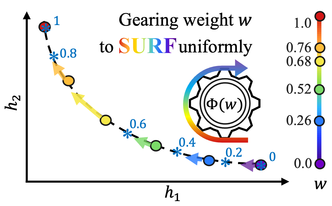
The paper’s bandit example compares points produced by uniform weights with points from geometry-aware sampling. Even spacing in weight space does not imply even spacing on the Pareto front.
Original paper source

Appendix F.1 / exact gear toy

Change traversal, keep the same front

Here x is a scalar decision, w weights the first raw objective, and p is the gear parameter. The raw objectives $h_1^p(x)$ and $h_2(x)$ select $x_w^*$ . The fixed evaluation vector $\bar{\mathbf h}(x)$ traces the same front as p changes.

\begin{aligned}h_1^p(x)&=\frac{\sqrt p}{2}(x-1)^2\\h_2(x)&=\frac{x^2}{2}\\x_w^*&=\frac{\sqrt p\,w}{1+(\sqrt p-1)w}\\\bar{\mathbf h}(x)&=\bigl((1-x)^2,x^2\bigr)\end{aligned}

Gear parameter p9

Front segments N9

Uniform weightsUniform arc length

N segments give $N+1$ solutions. This Appendix F.1 example uses the exact scalarized solution and direct numerical arc-length inversion. SURF’s iterative reconstruction is described in the method section.

A set of differently aligned summarization adapters

The LLM experiment trains six adapters representing different balances between summarization-quality and factual-faithfulness rewards. SURF reallocates the four intermediate weights while retaining the endpoint policies and the per-slot PPO budget. Its lower spacing CV corresponds to a more evenly distributed set of objective-space trade-offs.

Coverage and front quality in reinforcement learning and LLM alignment

Reddit summarization: coverage of quality–faithfulness trade-offs

Table 2 · KL-regularized objectives · mean ± standard deviation
Method	Hypervolume ↑	Spacing CV ↓	Gap ratio ↓
Uniform-w	3.76 ± 0.31	0.65 ± 0.12	5.89 ± 1.15
SURF	4.03 ± 0.35	0.30 ± 0.17	2.93 ± 5.35

Result

With the same per-slot PPO budget, SURF reduces the mean spacing coefficient of variation and gap ratio while increasing mean hypervolume. CV measures the standard deviation of neighboring objective-space distances relative to their mean. The gap ratio divides the largest distance by the smallest, making it sensitive to unusually short segments in the stochastic evaluation.

Experiment setup and comparison details

Qwen2.5-0.5B-Instruct has a frozen backbone and trainable LoRA adapters. PPO optimizes summarization-quality and factual-faithfulness rewards with KL coefficient 0.05. $N=5$ segments gives six model slots. After a shared 10-epoch $w=0$ .5 warm start, Uniform-w trains each slot for 12 PPO epochs. SURF starts from each slot’s epoch-5 checkpoint and performs seven one-epoch outer updates; endpoint policies are reused from Uniform-w. Both methods therefore have the same 12-epoch per-slot budget. Table 2 evaluates 10 batches of 64 prompts and reports mean ± standard deviation across these batches. The displayed entries use KL-regularized objectives; reward-only entries appear separately in the paper.

Read the original result

Fishwood: spacing gains at similar front-approximation quality

Table 1 · original reported scales · mean ± standard deviation
Method	HV (×10⁻¹) ↑	IGD (×10⁻²) ↓	CV (×10⁻¹) ↓	Gap ratio ↓
Soup	2.39 ± 0	0.91 ± 0	2.00 ± 0	1.90 ± 0
Uniform-w	2.40 ± 0	0.91 ± 0	1.94 ± 0	1.75 ± 0
UMOD	2.39 ± 0.00	0.92 ± 0.00	2.33 ± 0.17	2.14 ± 0.14
OLS	2.39 ± 0	0.96 ± 0	3.57 ± 0	2.49 ± 0
SURF	2.39 ± 0	0.90 ± 0	0.26 ± 0	1.12 ± 0

Result

Hypervolume and IGD remain similar across methods on Fishwood. SURF reduces the reported CV from 1.94 to 0.26 on the table’s ×10⁻¹ scale relative to Uniform-w, and lowers the gap ratio from 1.75 to 1.12. This comparison separates coverage uniformity from front-approximation quality.

Experiment setup and comparison details

The Fishwood environment trades off fishing and wood-collection rewards. SURF uses $N=11$ segments, 15 outer iterations, and damping 0.3. Optimization-based methods receive the same total number of inner iterations. Table 1 reports mean ± standard deviation over eight realizations; zero standard deviation denotes a deterministic experiment.

Read the original result

Objective scaling determines the coverage metric

Equal arc length is defined in the chosen objective-space metric. Rescaling either objective changes that metric and therefore changes the allocation of weights. The geometric analysis specifies what uniform coverage means before constructing it.

Cite this work

@inproceedings{jiang2026surf,
  title = {SURF: Steering the Scalarization Weight to Uniformly Traverse the Pareto Front},
  author = {Liuyuan Jiang and Chentong Huang and Lisha Chen},
  booktitle = {Advances in Neural Information Processing Systems},
  year = {2026}
}

Summary

Why uniform weights produce uneven coverage

The coverage problem

The geometric cause

Geometry-aware weight allocation

Arc-length reconstruction and weight refinement

Scalarization geometry and convergence of SURF

Notation

An invertible arc-length map

Linear convergence to the discretization floor

Regularity of the scalarization path

From traversal speed to equal arc length

CDF convergence and spacing uniformity

Further details

Related projects

Weight spacing and Pareto-front spacing

Change traversal, keep the same front

A set of differently aligned summarization adapters

Coverage and front quality in reinforcement learning and LLM alignment

Reddit summarization: coverage of quality–faithfulness trade-offs

Fishwood: spacing gains at similar front-approximation quality

Objective scaling determines the coverage metric

Cite this work

Research sources